This article is more than 1 year old
Hands on with MDX
Dimension and measures (yes, but can it handle cubic furlongs?)
Following our introduction to MDX (to be found here) this follow-up article is a get-you-started guide to using this powerful language to manipulate multi-dimensional data.
The basics
Relational databases store data in two-dimensional tables, a familiar concept that mimics grids of data on paper. Multi-dimensional data is fundamentally different and is stored as dimensions and measures. Dimensions describe the data: examples are Products (the items we sell), Location (where sales take place) and Time. Measures are usually numeric, like Units Sold, Sales and Budget.
We can see the principle of multi-dimensional data in a very simple two-dimensional structure. Here there are two descriptive dimensions – Products in the rows and Time in the columns. There is one numerical measure, Units Sold.
Units Sold
| Jan | Feb | Mar | Apr | |
|---|---|---|---|---|
| Apples | 125 | 45 | 78 | 169 |
| Figs | 74 | 53 | 89 | 39 |
| Lemons | 20 | 21 | 25 | 14 |
| Pears | 220 | 74 | 103 | 156 |
But, unlike tables in a relational database, we aren’t limited to two dimensions. Add a third – Location - and we get a 3-D cube of data.
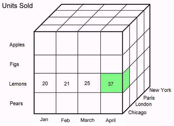
As before the rows show Products and the columns show Time. The slices that give the cube depth show the additional Location dimension. The values held at the intersections of all three dimensions are the Units Sold. (For simplicity only four values are shown). The green cell shows the number of lemons sold in Chicago in April.
Dimensions contain members and here each dimension has four: Chicago, London, Paris and New York are the four members in the Location dimension.
A multi-dimensional data structure can have many more dimensions, and this is where any visualisation technique breaks down. We humans live in a 3-D world and imagining further dimensions is hard: however, the cube analogy is a good starting point for understanding the principle behind multi-dimensional structures. (Not entirely coincidentally, multi-dimensional OLAP structures are commonly called cubes).
Hierarchies, levels and aggregations
Dimensions are often hierarchical which enables them to hold data at different levels. A Time dimension is almost invariably hierarchical and typical levels might be years, quarters and months.
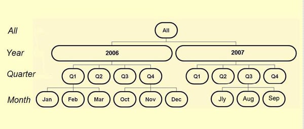
Hierarchies usually have an All level at the top to give a grand total of all data, with levels below. In this case the Year level contains members for 2006 and 2007, each of these is divided into four quarters and each quarter into three months. (Not all the months are shown.) This hierarchy lets us look at the Units Sold measure for each time period: all fig sales in a particular year, quarter or month.
During the cube-building process, data for the lowest level, called the leaf level (monthly values here but could be weekly, daily, whatever) is combined to give the higher values, quarters combine into years, and years into All. These calculated values are called aggregations.
